Subsonic turbulent flow of Mach 0.2, Reynolds number 5 million over a flat plate

Problem Statement

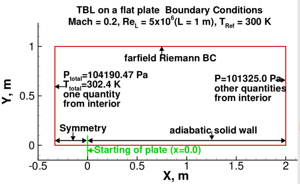
In this test case, a subsonic turbulent flow of Mach 0.2 over a flat plate will be simulated. The domain used, and boundary condition applied to the domain are illustrated in Fig. 1. The case definition and grid used were obtained from Turbulence Modeling Resource.

Mesh

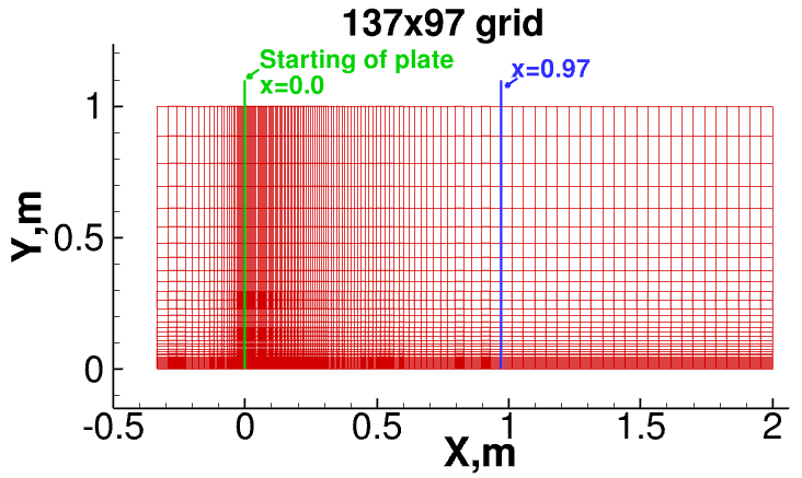
A structured grid of size 113 × 81 x 2 will be used as shown in Fig. 3. The grid is available in the tutorial folder |rootFolder|/run/Tutorial/TurbulentFlatPlate/CreateBlocks/.

In the blocking_point.f90 edit the number of blocks in the I-direction and J-direction. In this test case, four blocks will be used.
integer, parameter :: xblocks = 4
integer, parameter :: yblocks = 1
To compile the blocking_point.f90 code with gfortran and execute it, commands are written in the makefile. Just use the following command to generate grid files in the grid/ folder.

$make

Run the previous command in the |rootFolder|/run/Tutorial/TurbulentFlatPlate/CreateBlocks/ directory.

Setup

To set up the case directory, a python automation script is provided: automaton.py. First, set up the most important parameters, the paths to the grid files and main executable binary to FEST-3D
RunDir = 'FlatPlate_Turb' Name of the run directory to create for the current case.
GridDir= 'CreateBlocks/grid/' Path to the folder which only contains the grid files.
NumberOfBlocks = 4 Total number of blocks. It should match with the number of grid files available in the GridDir folder

AbsBinaryPath="/home/usr/FEST3D/bin/FEST3D"

Absolute path to the FEST-3D binary. Should be in |rootfolder|/bin/FEST3D
Now provide the common control parameters.
Control['CFL'] = 100.0 High CFL since implicit time-integration method will be used.
Control['LoadLevel'] = 0Since simulation will be started from scratch, 0 is specified.
Control['MaxIterations'] = 10000 Maximum number of iteration to perform.
Control['SaveIterations'] = 1000 Solution folder will be written every 1000 iteration.
Control['OutputFileFormat'] = 'vtk' Type of solution file to write. If you have tecplot file viewer you can user tecplot instead of vtk
Control['Purge'] = 1 Only one latest solution folder will be kept in the time_directories and rest will be deleted.
Control['ResidualWriteInterval'] = 20Write residual in time_directories/aux/resnorm after every 5 iteration.
Control['Tolerance'] = "1e-13 Continuity_abs" Stop the iteration if the absolute residual value of continuity equation is less than 1e-13.
Few scheme parameters for inviscid flow:
Scheme['InviscidFlux'] = 'ausm' Inviscid flux-reconstruction shceme. You can use: slau, ldfss0, ausmP , and ausmUP instead of __ausm.
Scheme['FaceState'] = 'muscl' Higher-order face-state reconstruction method. you can use: none, ppm, and weno.
Scheme['Limiter'] = '0 0 0 0 0 0' Switch off the limiter for I,J,and K direction and switch of pressure based switching for all direction.
Scheme['TurbulenceLimiter'] = '1 1 1' Using limiter only for turbulent variables face-state reconstruction improve convergence.
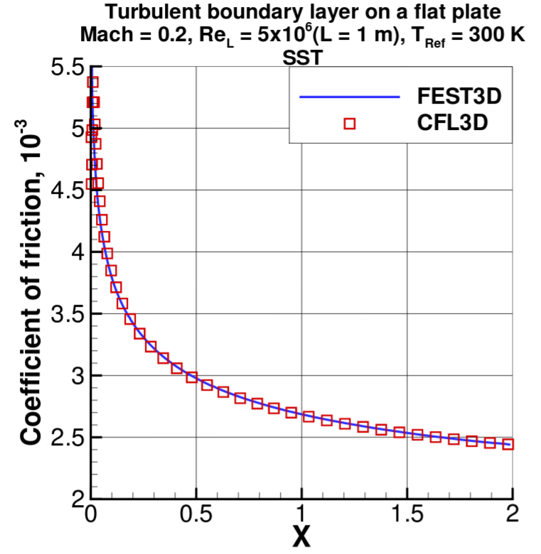
Scheme['TurbulenceModel']='sst' using SST turbulence model. Other models kkl, sa, and sst2003 can be user also.
Scheme['TransitionModel']='none' none is metioned for no transition model.
Scheme['TimeStep']='l' Local time stepping method. You can use global time-stepping method also g.
Scheme['TimeIntegration']='implicit' LU-SGS matrix-free time integration method.
Now, lets define the flow feature of test case:
Flow["DensityInf"] = 1.17659 Free-stream density.
Flow["UInf"] = 69.445 Free-stream x-component of velcotiy vector. (Mach = 0.5 at T_ref=300K)
Flow["VInf"] = 0.0 Free-stream y-component of velcotiy vector.
Flow["WInf"] = 0.0 Free-stream z-component of velcotiy vector.
Flow["PressureInf"] = 101325.0 Free-stream pressure.
Flow["ReferenceViscosity"] = 1.63416586e-5 Reference viscosity is set such that the Reynolds number (L_ref=1m) is 5 million

OutputControl['Out'] = ["Velocity", "Density", "Pressure", "Mu"] Variables to write in the output file.
ResidualControl['Out'] = ["Mass_abs", "Viscous_abs", "Continuity_abs"] Residual to write in the resnorm file.
BoundaryConditions = [-8, -4, -5, -6, -6, -6] Broad boundary condition.[Riemann inlet, subsonic outlet, no-slip wall and slip wall for rest ]. Since the bottom faces of the full domain have two different boundary conditions, as shown in Fig. 1, and the blocking provided here is such that first out the four blocks have inviscid region as a boundary condition at the bottom face and other three have the no-slip adiabatic wall as a boundary condition at the bottom faces. The boundary condition at the bottom face (Jmin) will be changed manually in the layout.md file after the automatic case setup.

Rest of the variables should be left to their default value. To execute this script, use the following command:

$python automaton.py

Now you will see a new folder created with RunDir name (FlatPlate_Turb). Switch to that directory to run the test case. To make sure setup is correct, check the layout.md file located in system/mesh/layout/layout.md. The file should look like the following:

## BLOCK LAYOUT FILE
## ==========================
## NUMBER OF PROCESSES
4
## NUMBER OF ENTRIES PER PROCESS
9
## PROCESS_NO GRID BC_FILE IMIN IMAX JMIN JMAX KMIN KMAX
## ===================================
## PROCESS 0
00  grid_00.txt  bc_00.md  -008  0001  -005  -006  -006  -006
## PROCESS 1
01  grid_01.txt  bc_01.md  0000  0002  -005  -006  -006  -006
## PROCESS 2
02  grid_02.txt  bc_02.md  0001  0003  -005  -006  -006  -006
## PROCESS 3
03  grid_03.txt  bc_03.md  0002  -004  -005  -006  -006  -006

Change the Jmin boundary condition for the first block from no-slip wall (-5) to slip wall (-6).

## BLOCK LAYOUT FILE
## ==========================
## NUMBER OF PROCESSES
4
## NUMBER OF ENTRIES PER PROCESS
9
## PROCESS_NO GRID BC_FILE IMIN IMAX JMIN JMAX KMIN KMAX
## ===================================
## PROCESS 0
00  grid_00.txt  bc_00.md  -008  0001  -006  -006  -006  -006
## PROCESS 1
01  grid_01.txt  bc_01.md  0000  0002  -005  -006  -006  -006
## PROCESS 2
02  grid_02.txt  bc_02.md  0001  0003  -005  -006  -006  -006
## PROCESS 3
03  grid_03.txt  bc_03.md  0002  -004  -005  -006  -006  -006

Finally, to run the simulation use the following command:

$nohup bash run.sh &

nohup helps in avoiding any output on the screen, & execute the last command in the background, allowing you to keep using the terminal.

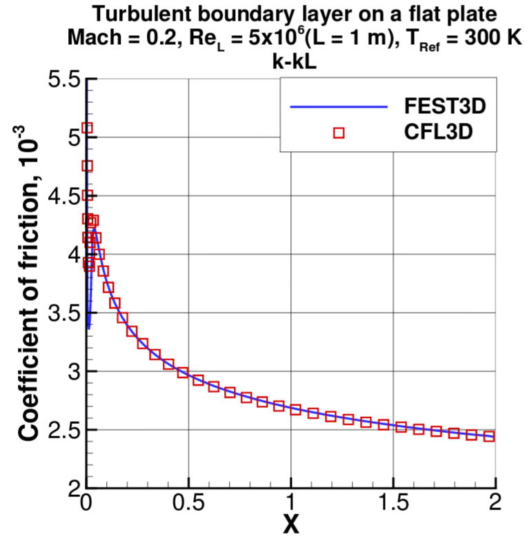
Results