Lid-Driven Cavity
Lid-driven cavity
Problem Statement
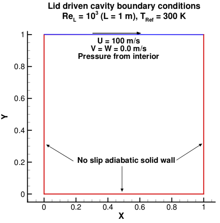
In this test case, we calculate the flow inside the cavity formed simulated due to the tangential velocity of the upper plate
. The domain used, and boundary condition applied to the domain are illustrated in Fig. 2.
The case definition and grid used were obtained from
NPARC Alliance Validation Archive.
Mesh
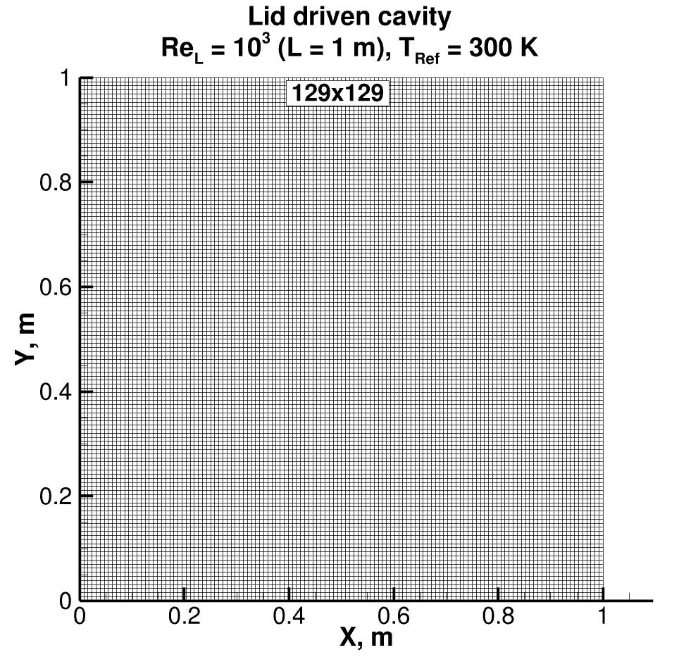
A uniform structured grid of size 129 x 129 × 2 will be used as shown in Fig. 3. The grid is available in the tutorial folder |rootFolder|/run/Tutorial/LidDrivenCavity/CreateBlocks/.
Note
If run folder is empty, please download the content from Github
direcotry or download the zip file here.
In the blocking_point.f90
edit the number of blocks in the I-direction and J-direction. In this test case, four blocks will
be used.
integer, parameter :: xblocks = 2
integer, parameter :: yblocks = 2
In order to compile the blocking_point.f90 code with gfortran and execute it, commands are written
in the makefile. Just use the following command to generate grid files in the grid/ folder.
$make
Run the previous command in the |rootFolder|/run/Tutorial/LidDrivenCavity/CreateBlocks/ directory.
Note
Make sure you are using numpy version greater than 1.10 for python script to generate grid.
Setup
To setup the case directory, a python automation script is provided: automaton.py. First setup the most important
parameters, the paths to the grid files and main executable binary to FEST-3D
RunDir = 'GiveAnyName' Name of the run directory to create for current case.
GridDir= 'CreateBlocks/grid/' Path to the folder which only contains grid file.
NumberOfBlocks = 4 Total number of blocks. It should match with number of gridfiles avaiable in the GridDir folder
AbsBinaryPath="/home/usr/FEST3D/bin/FEST3D"
Absolute path to the FEST-3D binary. Should be in |rootfolder|/bin/FEST3D
Now provide the common control parameters.
Control['CFL'] = 10.0 High CFL since implicit time-integration method will be used.
Control['LoadLevel'] = 0Since simulation will be started from scratch, 0 is specified.
Control['MaxIterations'] = 10000 Maximum number of iteration to perform.
Control['SaveIterations'] = 1000 Solution folder will be written every 1000 iteration.
Control['OutputFileFormat'] = 'vtk' Type of solution file to write. If you have tecplot file viewer you can user tecplot instead of vtk
Control['Purge'] = 1 Only one latest solution folder will be kept in the time_directories and rest will be deleted.
Control['ResidualWriteInterval'] = 20Write residual in time_directories/aux/resnorm after every 5 iteration.
Control['Tolerance'] = "1e-13 Continuity_abs" Stop the iteration if the absolute residual value of continuity equation is less than 1e-13.
Few scheme parameters for inviscid flow:
Scheme['InviscidFlux'] = 'slau' Inviscid flux-reconstruction shceme. You can use: ausm, ldfss0, ausmP , and ausmUP instead of __slau.
Scheme['FaceState'] = 'ppm' Higher-order face-state reconstruction method. you can use: none, muscl, and weno.
Scheme['Limiter'] = '0 0 0 0 0 0' Switch off the limiter for I,J,and K direction and switch of pressure based switching for all direction.
Scheme['TimeStep']='g 1e-5' Global time-stepping method and time-step. You can use local time-stepping method also l.
Scheme['TimeIntegration']='implicit' LU-SGS matrix-free time integration method.
Now, lets define the flow feature of test case:
Flow["DensityInf"] = 1.2 Free-stream density.
Note
The domain is initialized with zero velocity vector and Lid velocity is defined later in the boundary condition file. As the residual are normalized with free-stream velocity, residual written in resnom file will be Nan. But solution is correct.
Flow["UInf"] = 0.0 Free-stream x-component of velcotiy vector.
Flow["VInf"] = 0.0 Free-stream y-component of velcotiy vector.
Flow["WInf"] = 0.0 Free-stream z-component of velcotiy vector.
Flow["PressureInf"] = 103338.0 Free-stream pressure.
Flow["ReferenceViscosity"] = 1.2e-1 Reference viscosity is set to 0.12 so that the Reynolds number based on the lid-velocity (100m/s) is 1000
OutputControl['Out'] = ["Velocity", "Density", "Pressure", "Mu"] Variables to write in the output file.
ResidualControl['Out'] = ["Mass_abs", "Viscous_abs", "Continuity_abs"] Residual to write in the resnorm file.
BoundaryConditions = [-5, -5, -5, -3, -6, -6] Broad boundary condition.[Noslip adiabatic side and lower wall, and upper wall with slip velocity of 100 m/s ]. The velocity at the upper wall is set manually, later, in the bc_02.md and bc_03.md boundary condition file.
Rest of the variables should be left to their default value. In order to execute this script use following command:
$python automaton.py
Now you will see a new folder created with RunDir name. Switch to that directory to run the test case. To make sure setup is correct, check
the layout.md file located in system/mesh/layout/layout.md. The file should look like the following:
## BLOCK LAYOUT FILE
## ==========================
## NUMBER OF PROCESSES
4
## NUMBER OF ENTRIES PER PROCESS
9
## PROCESS_NO GRID BC_FILE IMIN IMAX JMIN JMAX KMIN KMAX
## ===================================
## PROCESS 0
00  grid_00.txt  bc_00.md  -005  0001  -005  0002  -006  -006
## PROCESS 1
01  grid_01.txt  bc_01.md  0000  -005  -005  0003  -006  -006
## PROCESS 2
02  grid_02.txt  bc_02.md  -005  0003  0000  -003  -006  -006
## PROCESS 3
03  grid_03.txt  bc_03.md  0002  -005  0001  -003  -006  -006
If all the boundary conditions are defined in the layout.md file then fix the upper wall velocity in the bc_02.md and bc_03.md file in system/mesh/bc/ folder. Change the bc_02.md file from
# jmx
- FIX_DENSITY
- FIX_X_SPEED
- FIX_Y_SPEED
- FIX_Z_SPEED
- COPY_PRESSURE
to
# jmx
- FIX_DENSITY
- FIX_X_SPEED 100.0
- FIX_Y_SPEED 0.0
- FIX_Z_SPEED 0.0
- COPY_PRESSURE
and same for bc_03.md file.
Finally, to run the simulation use the following command:
$nohup bash run.sh &
nohup helps in avoiding any output on the screen, & execute the last command in the background, allowing you to keep using the terminal.
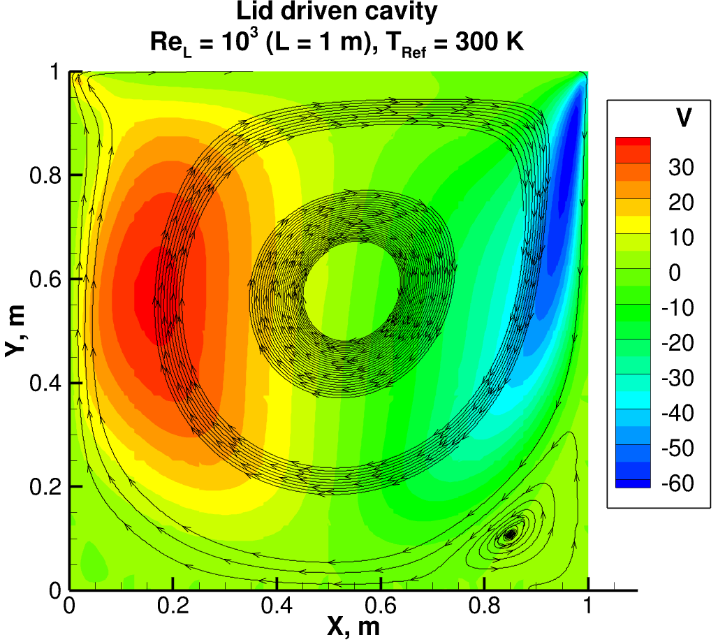
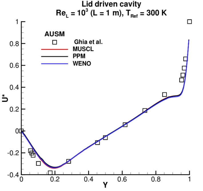
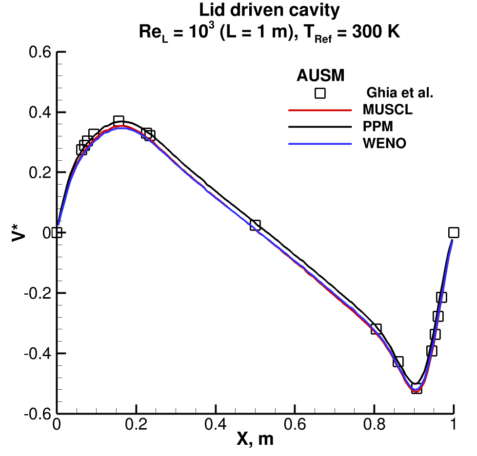
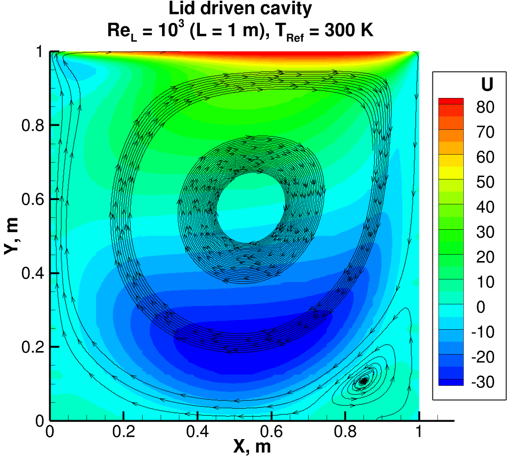
Results