2D Smooth Bump
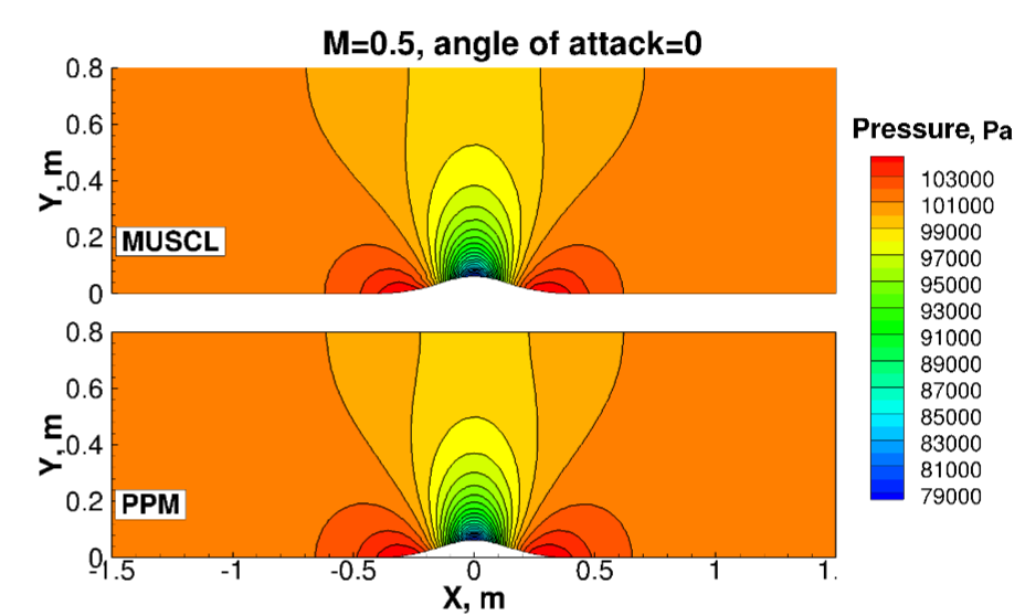
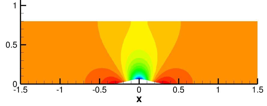
Subsonic inviscid flow of Mach 0.5 past a smooth 2D-bump
Problem Statement
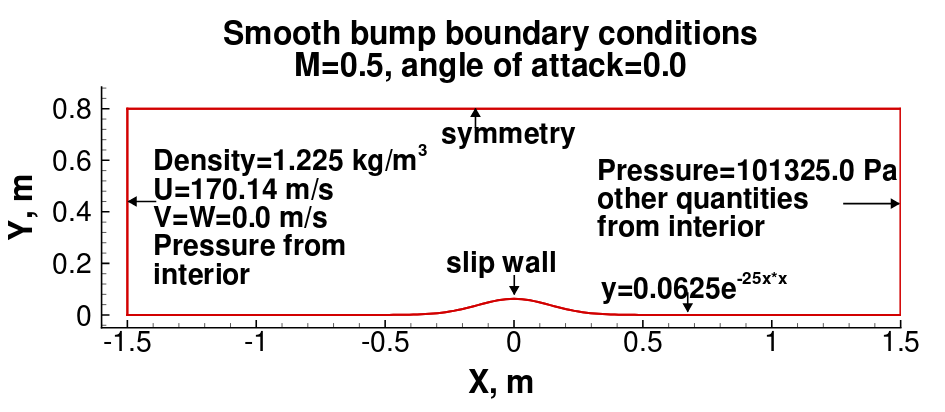
In this test case, a subsonic inviscid flow of Mach 0.5 past a smooth 2D-bump will be simulated. The domain used, and boundary
condition applied to the domain are illustrated in Fig. 2. The case definition and grid used were obtained from
4th International Workshop on High-Order CFD Methods .
Mesh
A structured grid of size 97 x 49 × 2 will be used, as shown in Fig. 3. The grid is available in the tutorial folder |rootFolder|/run/Tutorial/2DBump/CreateBlocks/.
Note
If run folder is empty, please download the content from Github
direcotry or download the zip file here.
In the bump.py
edit the number of blocks in the I-direction . In this test case, only two blocks will
be used.
imax = 97 Maximum number of grid points in the I-direction
jmax = 49 Maximum number of grid points in the J-direction
kmax = 2 Maximum number of grid points in the K-direction
blocks = 2 Number of blocks in the I-direction
In order to execute the bump.py script with python, all commands are written
in the makefile. Just use the following command to generate grid files in the grid/ folder.
$make
Run the previous command in the |rootFolder|/run/Tutorial/2DBump/CreateBlocks/ directory.
To setup the case directory, a python automation script is provided: Absolute path to the FEST-3D binary. Should be in |rootfolder|/bin/FEST3D Rest of the variables should be left to their default value. In order to execute this script use following command: Now you will see a new folder created with The last two uncommented line, in sequence, indicates following: Since there are two blocks, there are two rows of entries, one for each block. All the lines with 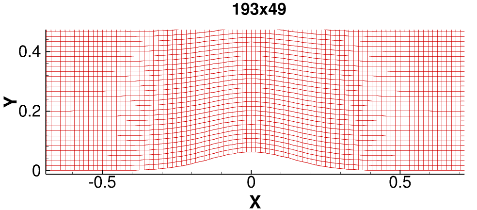
Setup
automaton.py. First setup the most important
parameters, the paths to the grid files and main executable binary to FEST-3D
RunDir = 'GiveAnyName' Name of the run directory to create for current case.
GridDir= 'CreateBlocks/grid/' Path to the folder which only contains grid file.
NumberOfBlocks = 2 Total number of blocks. It should match with number of gridfiles avaiable in the GridDir folder AbsBinaryPath="/home/usr/FEST3D/bin/FEST3D"
Now provide the common control parameters.
Control['CFL'] = 10.0 High CFL since implicit time-integration method will be used.
Control['LoadLevel'] = 0Since simulation will be started from scratch, 0 is specified.
Control['MaxIterations'] = 10000 Maximum number of iteration to perform.
Control['SaveIterations'] = 1000 Solution folder will be written every 1000 iteration.
Control['OutputFileFormat'] = 'tecplot' Type of solution file to write. If you have vtk file viewer you can user vtk instead of tecplot
Control['Purge'] = 1 Only one latest solution folder will be kept in the time_directories and rest will be deleted.
Control['ResidualWriteInterval'] = 5Write residual in time_directories/aux/resnorm after every 5 iteration.
Control['Tolerance'] = "1e-13 Continuity_abs" Stop the iteration if the absolute residual value of continuity equation is less than 1e-13.
Few scheme parameters for inviscid flow:
Scheme['InviscidFlux'] = 'slau' Inviscid flux-reconstruction shceme. You can use: ausm, ldfss0, ausmP , and ausmUP instead of __slau.
Scheme['FaceState'] = 'muscl' Higher-order face-state reconstruction method. you can use: none, ppm, and weno.
Scheme['Limiter'] = '0 0 0 0 0 0' Switch on the limiter for I,J,and K direction and switch of pressure based switching for all direction.
Scheme['TimeStep']='l' Local time-stepping method. You can use global time-stepping method also g.
Scheme['TimeIntegration']='implicit' LU-SGS matrix-free time integration method.
Now, lets define the flow feature of test case:
Flow["DensityInf"] = 1.225 Free-stream density.
Flow["UInf"] = 170.14 Free-stream x-component of velcotiy vector.
Flow["VInf"] = 0.0 Free-stream y-component of velcotiy vector.
Flow["WInf"] = 0.0 Free-stream z-component of velcotiy vector.
Flow["PressureInf"] = 101325.0 Free-stream pressure.
Flow["ReferenceViscosity"] = 0.0 Set reference viscosity to zero for inviscid flow.OutputControl['Out'] = ["Velocity", "Density", "Pressure"] Variables to write in the output file.
ResidualControl['Out'] = ["Mass_abs", "Viscous_abs", "Continuity_abs"] Residual to write in the resnorm file.
BoundaryConditions = [-8, -4, -6, -6, -6, -6] Broad boundary condition.[Riemann-inlet, subsonic outlet, rest are Slip-walls]. Free-stream pressure is used to fix the pressure outlet value.$python automaton.py
RunDir name. Switch to that directory to run the test case. To make sure setup is correct, check
the layout.md file located in system/mesh/layout/layout.md. The file should look like the following:## BLOCK LAYOUT FILE
## ==========================
## NUMBER OF PROCESSES
2
## NUMBER OF ENTRIES PER PROCESS
9
## PROCESS_NO GRID BC_FILE IMIN IMAX JMIN JMAX KMIN KMAX
## ===================================
## PROCESS 0
00 grid_00.txt bc_00.md -008 0001 -006 -006 -006 -006
## PROCESS 1
01 grid_01.txt bc_01.md 0000 -004 -006 -006 -006 -006
Block_Number GridFile Boundary_condition_file Imin_boundary_condition_number Imax_boundary_condition_number Jmin_boundary_condition_number Jmax_boundary_condition_number Kmin_boundary_condition_number Kmax_boundary_condition_number
# as the first character are skipped while reading by the FEST-3D solver.
All the positive numbers define the interface boundary condition, and negative numbers define the physical boundary conditions.
Finally, to run the simulation use following command:$nohup bash run.sh &
nohup helps in avoiding any output on the screen, & execute the last command in the background, allowing you to keep using the terminal.Results